Generative Models for Approximating Cardinality Sketches
Brian Tsan
UC Merced
btsan@ucmerced.edu
Advisor: Professor Florin Rusu
Table of Contents
- Recap
- Query Optimization Problem
- AGMS (Tug-of-War) Sketch
- Other Sketches
- Generative Models for Approximate Sketching
- Neural Networks
- Sum-Product Networks
- Summary & Conclusion
Section 1: Recap
Approximate Sketches (SIGMOD'24)
SELECT COUNT(*) FROM customers c JOIN orders o ON c.customer_id = o.customer_id
	WHERE c.age = 35 AND c.city = 'SF'
| Input Embeddings | |
|---|---|
| age | h(35) = 7 |
| city | h('SF') = 12 |
| customer_id | [MASK] |
Summary
✓Pros
- Efficient approximation
- Accurate sketches
- Fast queries
❌Cons
- Long training
- Large model size
- GPU-bottlenecked
the background
Section 2: Query Optimization Problem
Joins
Find all students enrolled in special seminar courses
SELECT s.name, e.student_id, c.course_name
FROM Students s
JOIN Enrollments e ON s.student_id = e.student_id
JOIN SpecialCourses c ON e.course_id = c.course_id
Joins
| ID | Name |
|---|---|
| 1 | Alice |
| 2 | Bob |
| 3 | Carol |
| 4 | Dave |
| 5 | Eve |
| SID | CID |
|---|---|
| 1 | 101 |
| 2 | 101 |
| 1 | 201 |
| 3 | 201 |
| 4 | 202 |
| 5 | 202 |
| 2 | 203 |
| 3 | 203 |
| 4 | 204 |
| 5 | 205 |
| ID | Course |
|---|---|
| 101 | CS101 |
| 201 | CS102 |
Plan A: Join Students First (Bad Plan)
Step 1: Students ⋈ Enrollments
| ID | Name |
|---|---|
| 1 | Alice |
| 2 | Bob |
| 3 | Carol |
| 4 | Dave |
| 5 | Eve |
| SID | CID |
|---|---|
| 1 | 101 |
| 2 | 101 |
| 1 | 201 |
| 3 | 201 |
| 4 | 202 |
| 5 | 202 |
| 2 | 203 |
| 3 | 203 |
| 4 | 204 |
| 5 | 205 |
Cost: 5 × 10 = 50 comparisons
Plan A: Join Students First (Bad Plan)
Step 1 Result: 10 intermediate rows
| Name | SID | CID |
|---|---|---|
| Alice | 1 | 101 |
| Bob | 2 | 101 |
| Alice | 1 | 201 |
| Carol | 3 | 201 |
| Dave | 4 | 202 |
| Eve | 5 | 202 |
| Bob | 2 | 203 |
| Carol | 3 | 203 |
| Dave | 4 | 204 |
| Eve | 5 | 205 |
Plan A: Join Students First (Bad Plan)
Step 2: Result ⋈ SpecialCourses
| Name | CID |
|---|---|
| Alice | 101 |
| Bob | 101 |
| Alice | 201 |
| Carol | 201 |
| Dave | 202 |
| Eve | 202 |
| Bob | 203 |
| Carol | 203 |
| Dave | 204 |
| Eve | 205 |
| ID | Course |
|---|---|
| 101 | CS101 |
| 201 | CS102 |
Cost: 10 × 2 = 20 comparisons
Plan A: Join Students First (Bad Plan)
Final Result: 4 rows
| Name | Course |
|---|---|
| Alice | CS101 |
| Bob | CS101 |
| Alice | CS102 |
| Carol | CS102 |
Plan B: Join SpecialCourses First (Good Plan)
Step 1: SpecialCourses ⋈ Enrollments
| ID | Course |
|---|---|
| 101 | CS101 |
| 201 | CS102 |
| SID | CID |
|---|---|
| 1 | 101 |
| 2 | 101 |
| 1 | 201 |
| 3 | 201 |
| 4 | 202 |
| 5 | 202 |
| 2 | 203 |
| 3 | 203 |
| 4 | 204 |
| 5 | 205 |
Cost: 2 × 10 = 20 comparisons
Plan B: Join SpecialCourses First (Good Plan)
Step 1 Result: Only 4 intermediate rows!
| SID | Course |
|---|---|
| 1 | CS101 |
| 2 | CS101 |
| 1 | CS102 |
| 3 | CS102 |
Plan B: Join SpecialCourses First (Good Plan)
Step 2: Result ⋈ Students
| SID | Course |
|---|---|
| 1 | CS101 |
| 2 | CS101 |
| 1 | CS102 |
| 3 | CS102 |
| ID | Name |
|---|---|
| 1 | Alice |
| 2 | Bob |
| 3 | Carol |
| 4 | Dave |
| 5 | Eve |
Cost: 4 × 5 = 10 comparisons
Much smaller intermediate result!
Plan B: Join SpecialCourses First (Good Plan)
Final Result: 4 rows
| Name | Course |
|---|---|
| Alice | CS101 |
| Bob | CS101 |
| Alice | CS102 |
| Carol | CS102 |
Why Join Ordering Matters
❌ Plan A: Bad Order
Cost: 5 × 10 = 50
Result: 10 rows
Cost: 10 × 2 = 20
Result: 4 rows
✓ Plan B: Good Order
Cost: 2 × 10 = 20
Result: 4 rows ← Early filter!
Cost: 4 × 5 = 10
Result: 4 rows
Why Join Ordering Matters
Plan B is 2.3× faster
- Join with selective tables first to filter early
- Smaller intermediate results = fewer comparisons in subsequent joins
- For large tables, the difference can be orders of magnitude
The Challenge: How can the query optimizer choose the best join order before execution?
→ We need cardinality estimation to predict intermediate result sizes!
The Query Optimization Problem
- Query optimizers need to estimate cardinality
- Cardinality = size of query result
- Poor estimates → Poor query plans → Slow queries
- Critical for joins and selections
Example: Wrong estimate leads to wrong join order
10x slower query execution!
The Independence Assumption
Traditional estimators assume columns are independent
Reality: Data is often correlated!
This assumption fails → Massive estimation errors
Traditional Approaches & Their Limitations
Histograms
- ✅ Work well for single columns
- ❌ Multivariate = exponential space
- ❌ Still assume independence
Machine Learning
- ✅ Multivariate distributions
- ❌ Training overhead
- ❌ Join estimation challenging
Enter: Sketches
Sketch: Compact probabilistic data structure
- Sub-linear space usage
- Fast updates and queries
- Theoretical accuracy guarantees
- Can handle joins naturally!
But... they're query-specific 😕
Section 3: Sketch Fundamentals
The Tug-of-War Metaphor
AGMS Sketch: Elements compete in a "tug-of-war"
Each color assigned to +1 or -1 team
Pairwise Independent Hashing
Hash function: $\xi: \mathbb{R} \rightarrow \{\pm 1\}$
The reason tug-of-war works:
$\mathbb{E}[\xi(i)\xi(j)] = \begin{cases} 0 & \text{if } i \neq j \\ 1 & \text{if } i = j \end{cases}$
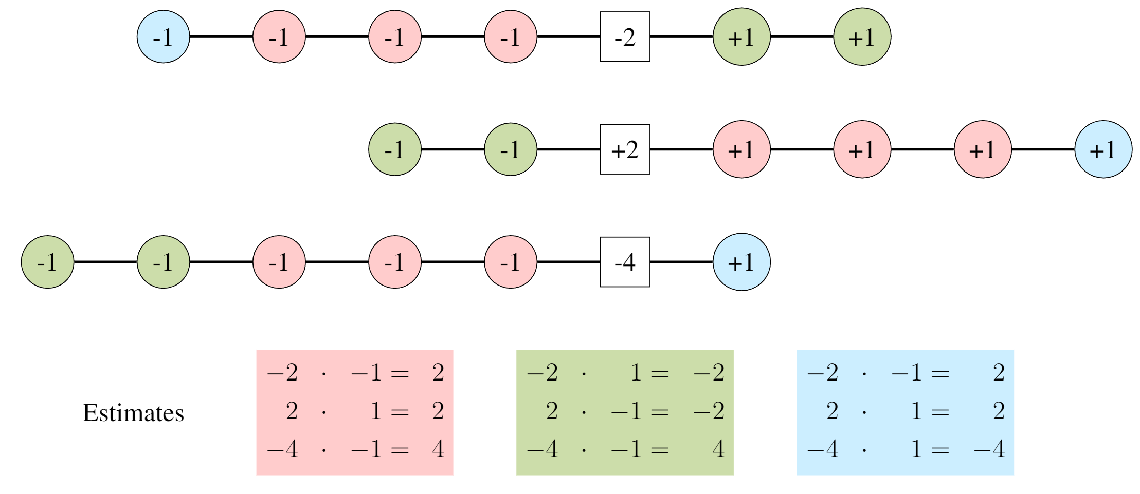
Point Selection Estimation
To estimate frequency of value $j$:
$f_j \approx s \cdot \xi(j)$
where $s = \sum_{i \in X} \xi(i)$ is the sketch
Unbiased! $\mathbb{E}[s \cdot \xi(j)] = f_j$
Variance: $\text{Var}[s \cdot \xi(j)] = F_2(X) - f_j^2$
AGMS Variance for frequency $f_j$
AGMS has high variance...
so you need to play a lot of tug-of-war!
Fast-AGMS: The Speed-Up
Use width-$w$ array instead of single counter
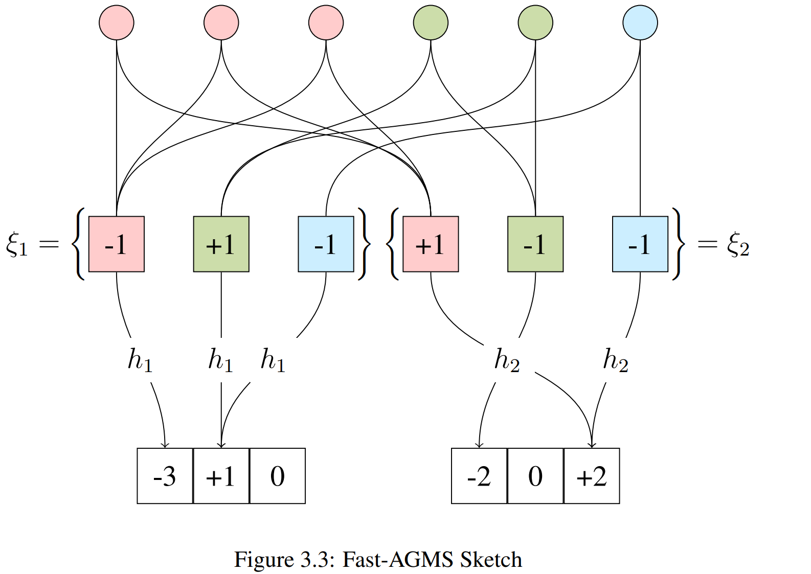
Each element goes to ONE counter → 1/w update time!
Range Queries: Dyadic Intervals
How to handle range predicates?
Decompose range into dyadic intervals!
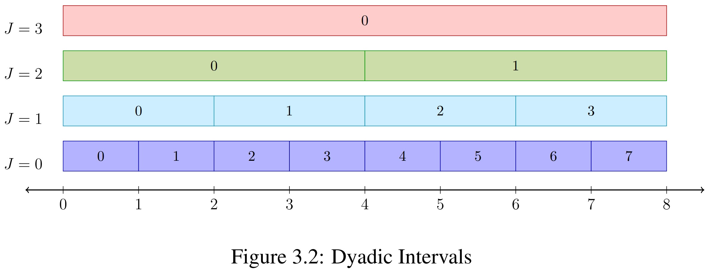
Any range decomposes into ≤ $2(\log_2(b-a) - 1)$ intervals
Join Cardinality Estimation
For join $X \bowtie Y$:
$|X \bowtie Y| \approx S_X \cdot S_Y$
Dot product of sketch vectors!
$T_1 \bowtie T_2 \bowtie T_3$
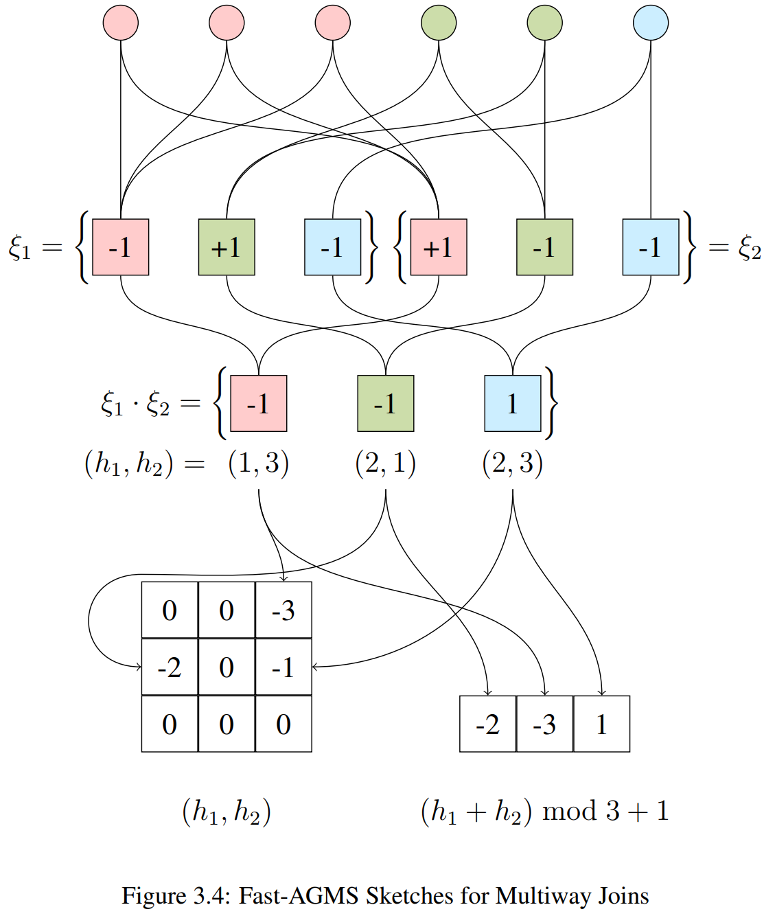
This generalizes to sktech tensors for more joins
But tensor size grows exponentially...
Efficient Multiway Joins: FFT
Avoiding Tensors with Circular Convolution
- Tensor size grows exponentially ($N^{\text{cols}}$)
- Convolution theorem: $A * B = \mathcal{F}^{-1}(\mathcal{F}(A) \cdot \mathcal{F}(B))$
- Compute in $O(N \log N)$ using Fast Fourier Transform!
Section 4: Other Sketches
Count-Min Sketch
Simplified: Always increment (no $\xi$ hash)
Trade-off: Biased (overestimates), but simpler & faster
Bound Sketch: Tighter Bounds
Track maximum frequency per bucket
$\max_i f_i \leq \sum_i f_i$ → Tighter than Count-Min!
Sketch Properties Summary
| Sketch | Linear? | Unbiased? | Space | Update Time |
|---|---|---|---|---|
| AGMS | ✅ Yes | ✅ Yes | O(dw) | O(dw) |
| Fast-AGMS | ✅ Yes | ✅ Yes | O(dw) | O(2d) |
| Count-Min | ✅ Yes | ❌ No (upper bound) | O(dw) | O(d) |
| Bound | ❌ No | ❌ No (tighter bound) | O(dw) | O(d) |
d = # independent sketches, w = sketch width
Section 4: The Dissertation's Contribution
The Problem with Sketches
Issue 1: Selections + Joins
→ Would need exponential sketch tensors
Issue 2: Query-specific construction
→ Need to scan entire dataset for each query
Issue 3: Many queries = many sketches
→ Storage explosion for diverse workloads
Solution: Approximate Sketches
Idea: Use ML models to generate sketches on-demand
Train model on data
Learn joint distribution
Query arrives
Generate sketch instantly
No data scan required! ✨
Two Modeling Approaches
Neural Networks
- Transformers for attention
- Hardware accelerated
- High capacity
- Gradient descent training
Sum-Product Networks
- Probabilistic graphical model
- Tractable inference
- Fast training
- Interpretable structure
Both approaches: Learn distribution → Generate sketches
Novel Approximate Sketching Methods
The Limitation of Traditional Sketches
- Sketches must be built for specific selections
- Selection = table rows satisfying filter conditions
- Problem: Filters are specified at query time
Example Query:
SELECT COUNT(*)
FROM orders o JOIN customers c ON o.customer_id = c.id
WHERE o.year = 2024 AND c.region = 'West'
Need sketches for σyear=2024(orders) and σregion='West'(customers)
Three Approaches to the Problem
1. Pre-compute All Sketches
- Build sketches for every possible selection
- Issue: Exponential combinations
- 10 attributes × 100 values each = 10010 possibilities
- Infeasible!
2. Build at Query Time
- Filter data, then construct sketch
- Issue: Requires full table scan
- COMPASS (GPU-accelerated): still hundreds of ms
- High overhead!
Three Approaches to the Problem
3. Approximate Sketches ✓
- Train a model on the table (offline)
- At query time: model predicts the sketch
- Benefit: Fast inference (~5-10 ms)
- Practical for query optimization!
Approximation Pipeline
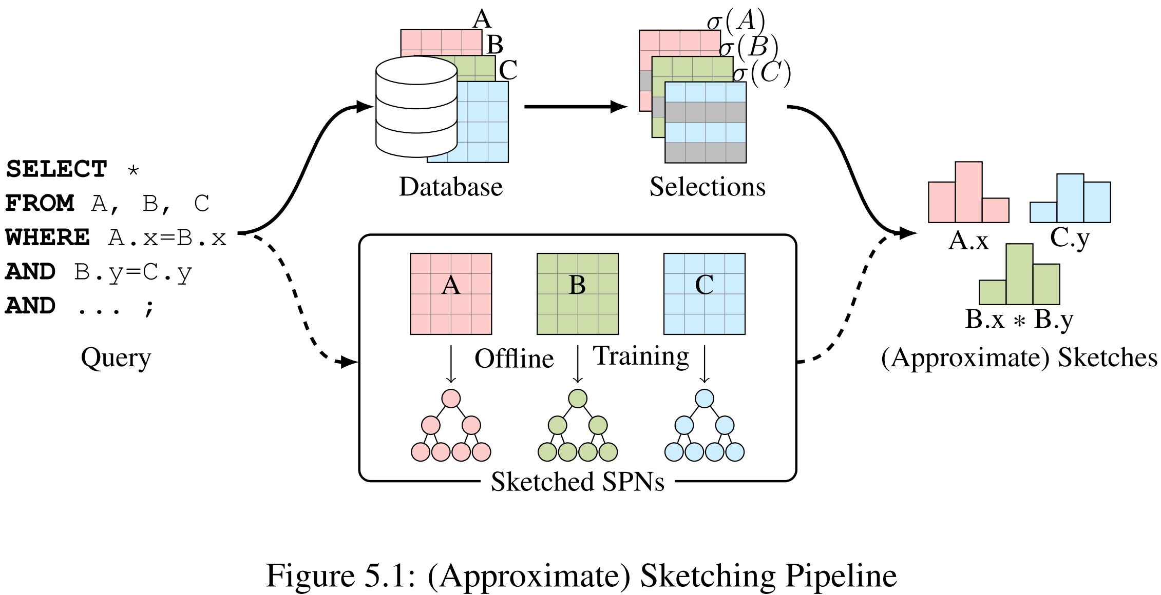
The exact sketching pipeline (top) is impractical.
Approximate Sketches (SIGMOD 2024)
Using Transformers to Approximate Count-Min Sketches
Probabilities into Sketches
A Count-Min sketch can be expressed as:
Where:
- p ∈ ℝw = probability mass distribution over hash bins
- |σφ(T)| = cardinality of the selection
- φ = filter predicates (e.g., age > 30 AND city = 'SF')
Idea: Train a model to estimate p for ANY predicate φ
Probabilities into Sketches
For a hash function h : ℝ → {1, ..., w}:
The i-th counter in the sketch:
= |σφ(T)| × P(h(X) = i | φ)
Therefore: sketch = p × |σφ(T)|
Transformer Architecture
SELECT COUNT(*) FROM customers c JOIN orders o ON c.customer_id = o.customer_id
WHERE c.age = 35 AND c.city = 'SF'
| Input Embeddings | |
|---|---|
| age | h(35) = 7 |
| city | h('SF') = 12 |
| customer_id | [MASK] |
Why Bidirectional Transformers?
Unidirectional (NeuroCard)
- Predicts P(Xi | X1, ..., Xi-1)
- Fixed column ordering
- Cannot condition on "future" columns
- Limitation: Sketch column must come after all filter columns
Bidirectional (BERT)
- Predicts P(Xi | all other Xj)
- No column ordering constraint
- Uses MASK tokens for prediction
- Advantage: Filters on ANY attributes work!
Essential for approximating sketches with arbitrary filter conditions
Training Data: Raw Table
Start with actual database table rows
| customer_id | age (point pred) |
city (point pred) |
year (range pred) |
|---|---|---|---|
| 1001 | 35 | 'SF' | 2022 |
| 1002 | 42 | 'NY' | 2019 |
| 1003 | 28 | 'LA' | 2021 |
| 1004 | 55 | 'SF' | 2023 |
Goal: Transform this data to train BERT to predict sketches for any filter condition
Training Pipeline
| Stage | Point Predicate (e.g., city) | Range Predicate (e.g., year) |
|---|---|---|
| 1. Raw Value | 'SF' | 2022 |
| 2. Dyadic Annotation | — | [2022,2023)2⁰, [2022,2024)2¹, ... |
| 3. Hash | h('SF') = 12 | h0 = 45, h1 = 28, ... |
| 4. Embedding | Map each hash to learnable vector in ℝd | |
| 5. Training | BERT masked language modeling: [h₁, h₂, [MASK], h₄] → predict h₃ | |
Join Cardinality Estimation Process
For query: SELECT * FROM A JOIN B ON A.x = B.y WHERE ...
-
Approximate Sketches:
- Model for A: infer sketch(σφ(A).x)
- Model for B: infer sketch(σψ(B).y)
-
Estimate Join:
- |A ⋈ B| ≈ sketch(A) · sketch(B)
- Take median of d independent estimates
SELECT COUNT(*) FROM customers c JOIN orders o ON c.customer_id = o.customer_id
WHERE c.age = 35 AND c.city = 'SF' AND o.year = 2023
city = 'SF'
Experimental Setup
Datasets:
- IMDb — 6 tables, 20 columns, up to 36M rows
- JOB-light: 70 queries
- JOB-light-ranges: 1000 queries
Baselines:
- Exact Fast-AGMS and Count-Min Sketches
- NeuroCard (Full Outer Join Transformer model)
Metrics
- Q-error: multiplicative error between estimated and true cardinality
- P-error: multiplicative error between plan cost of estimated and best plan
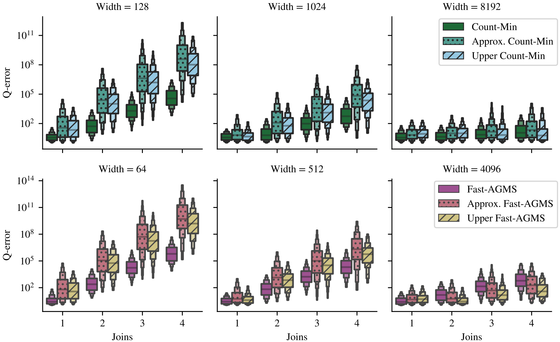
Q-error by Sketch Width
Estimation Time
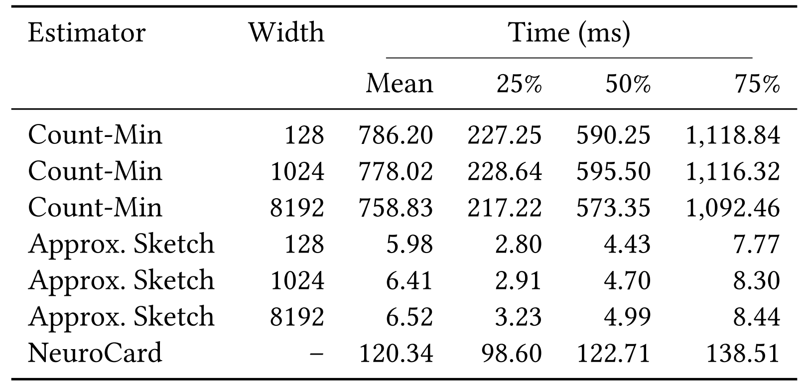
Approx. faster than exact (pushdown) sketches!
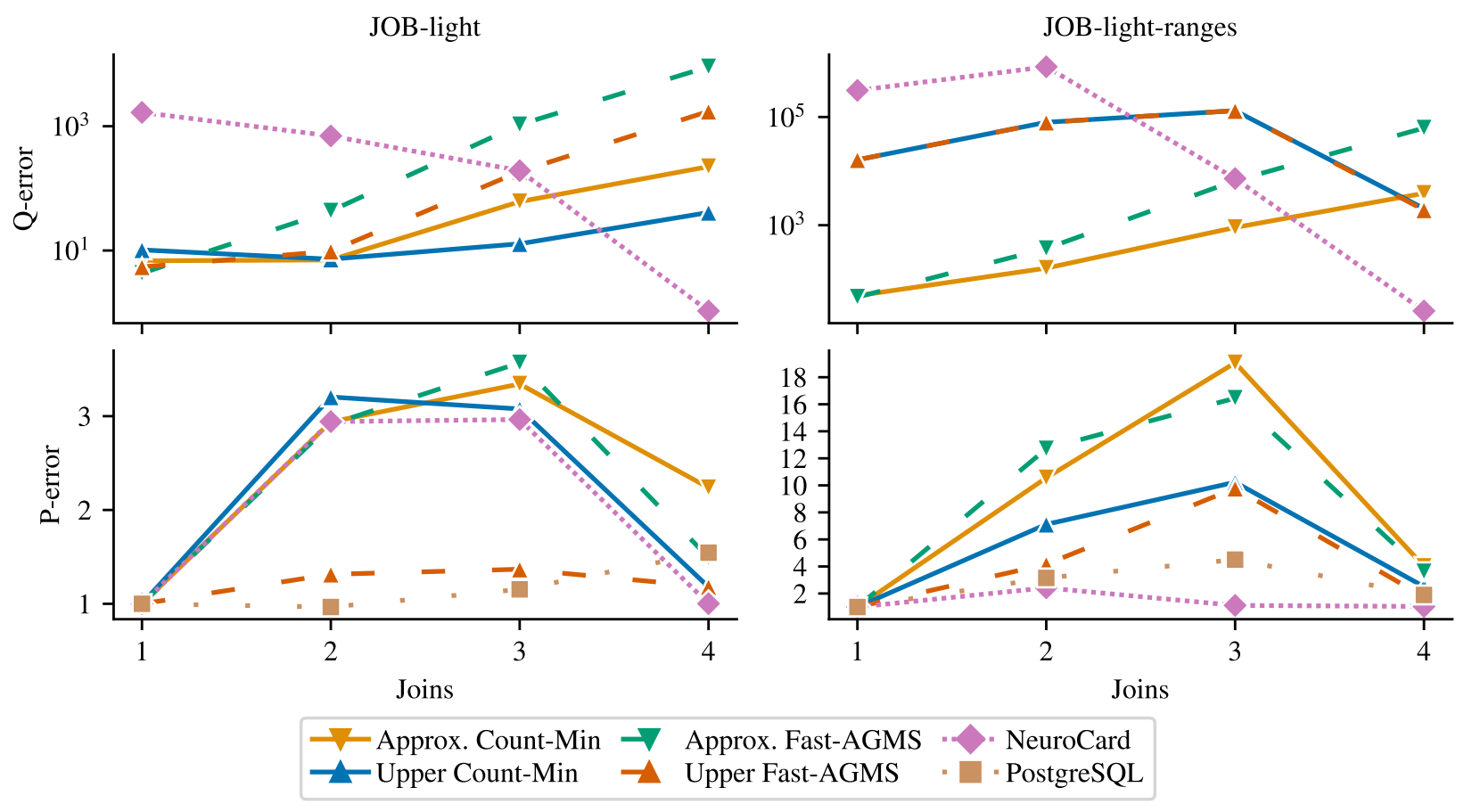
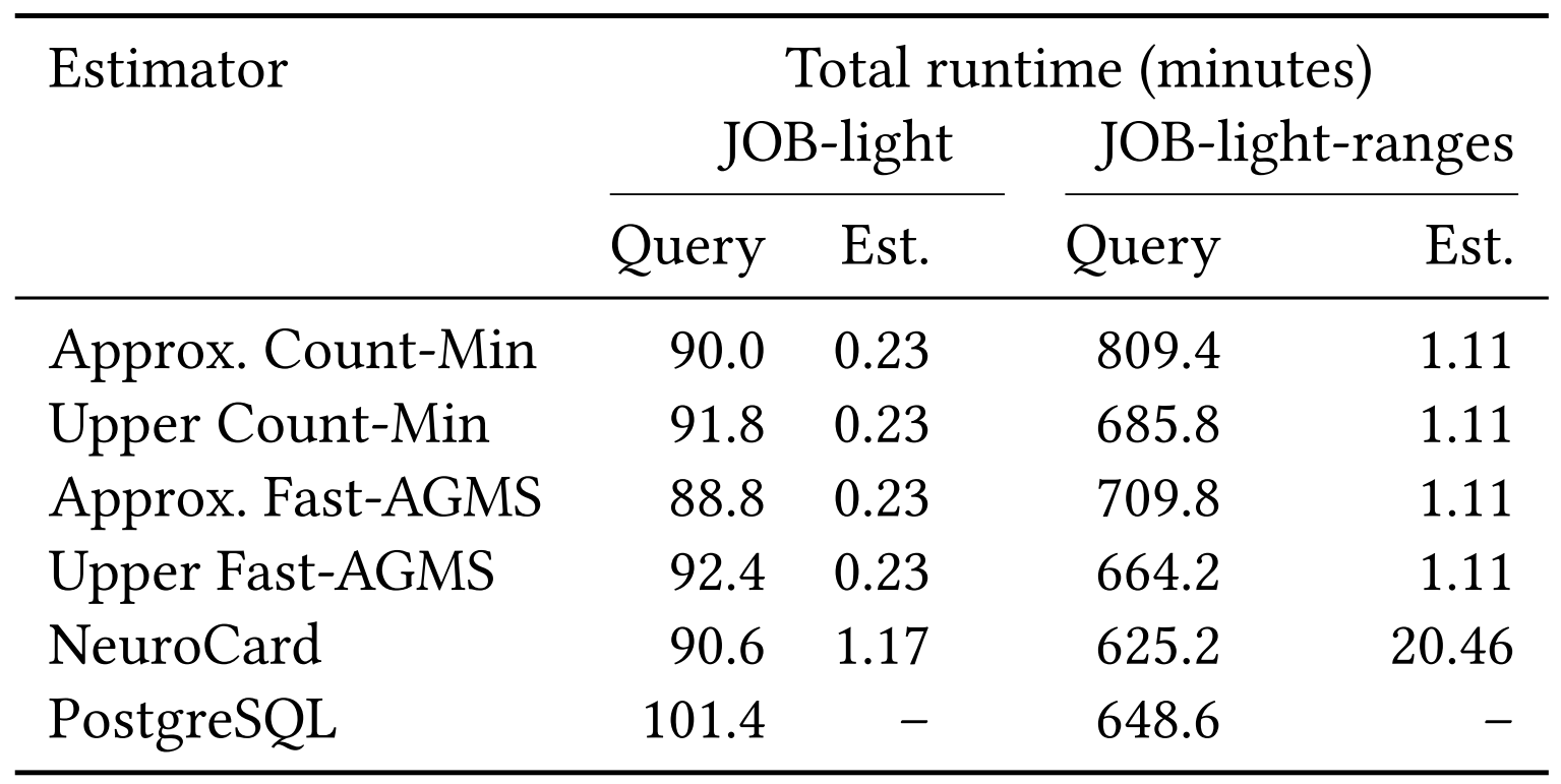
Q-error & P-error
Runtime
Limitations of Transformer Approach
-
Scalability Issue: Model size grows linearly with sketch width
- Need w × d × n embeddings (one per hash bin per attribute)
- GPU memory constraints limit practical width to ~4,096
-
Training Cost: Requires GPU acceleration
- 148 min/epoch on JOB-light (NVIDIA Tesla K80)
- Becomes prohibitive for larger sketches
- Problem: Larger sketches → better accuracy, but can't scale!
Sketched Sum-Product Networks (2025)
Scaling Beyond Transformer Limitations
What are Sum-Product Networks?
Trees made of:
- Sum nodes: Mixture of distributions (weighted average)
- Product nodes: Factorization of independent distributions
- Leaves: Simple univariate distributions
- Root: Represents full joint distribution
What are Sum-Product Networks?
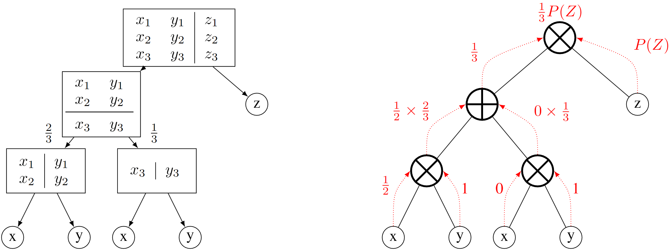
Training left, inference right
Training
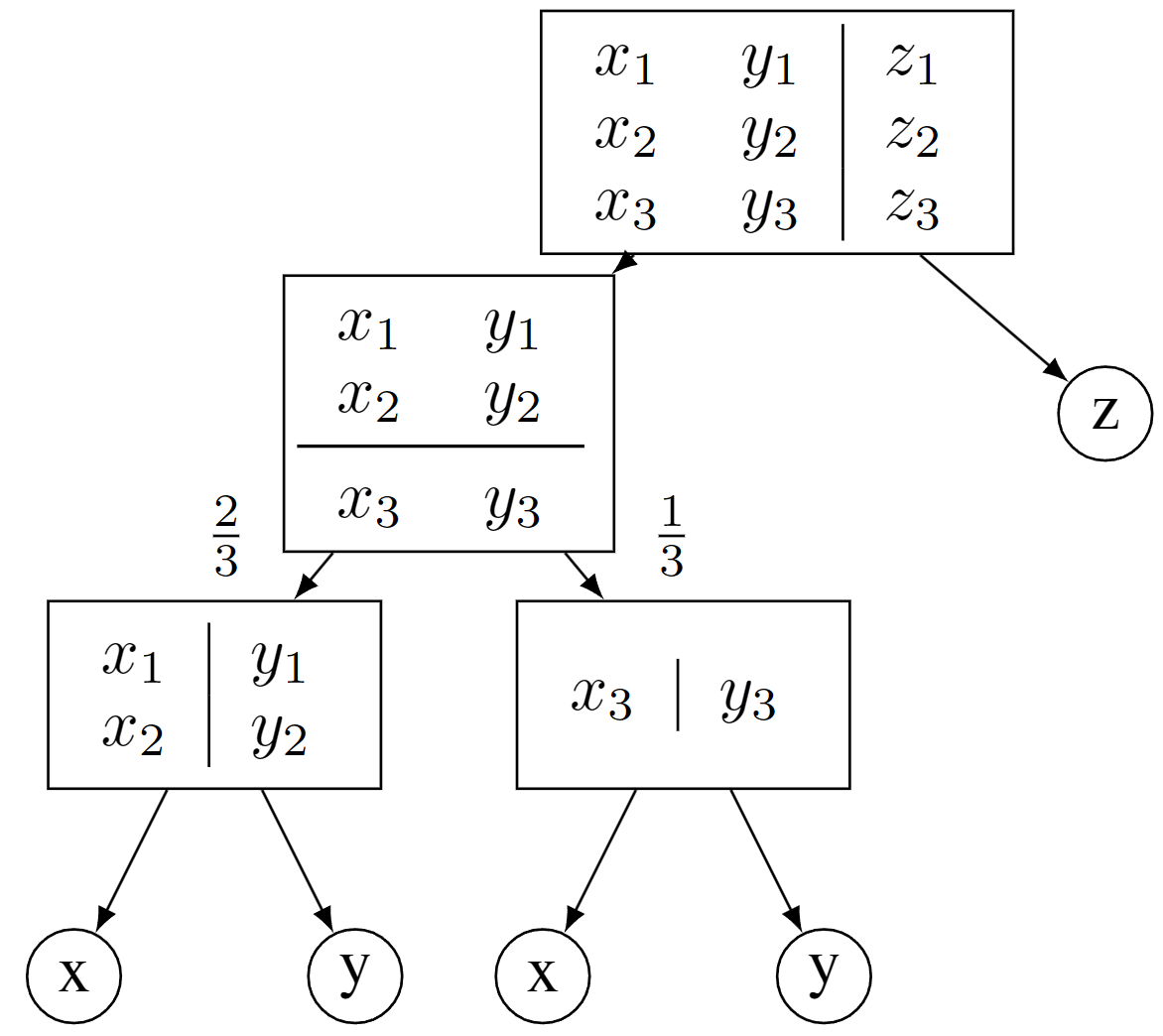
- One random variable
→ terminate (leaf node) - Independent variables
→ factorize (product node) - Otherwise
→ cluster (sum node)
Inference
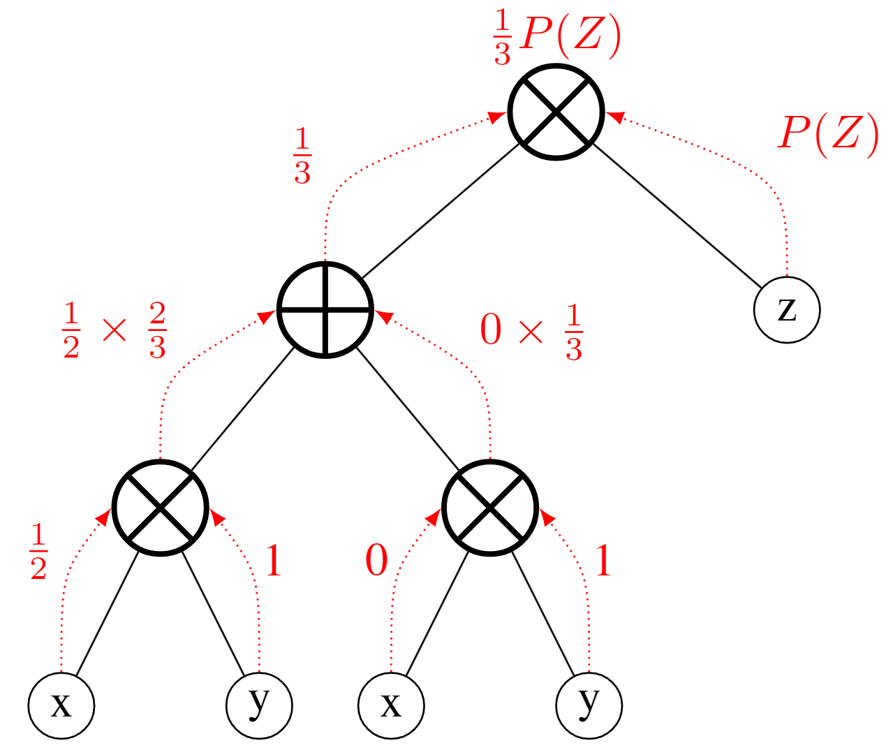
Query for
the distribution of $P(X, Z)$ where $X=x_2$
SPNs for Multivariate Data
Decompose complex joint distributions as linear combinations:
Advantages for Relational Data:
- Can handle mixed data types:
- both discrete & continuous
- Less than exponential storage
- No GPU required! Can train on CPU
Sketches from SPNs
Instead of storing probability distributions in leaf nodes...
Store sketches in leaf nodes!
- Each leaf represents a partition of the data
- Leaf stores the sketch of that partition
- Sketches combine via sum/product operations
- Result: Approximate sketch of any selection
Sketches from SPNs
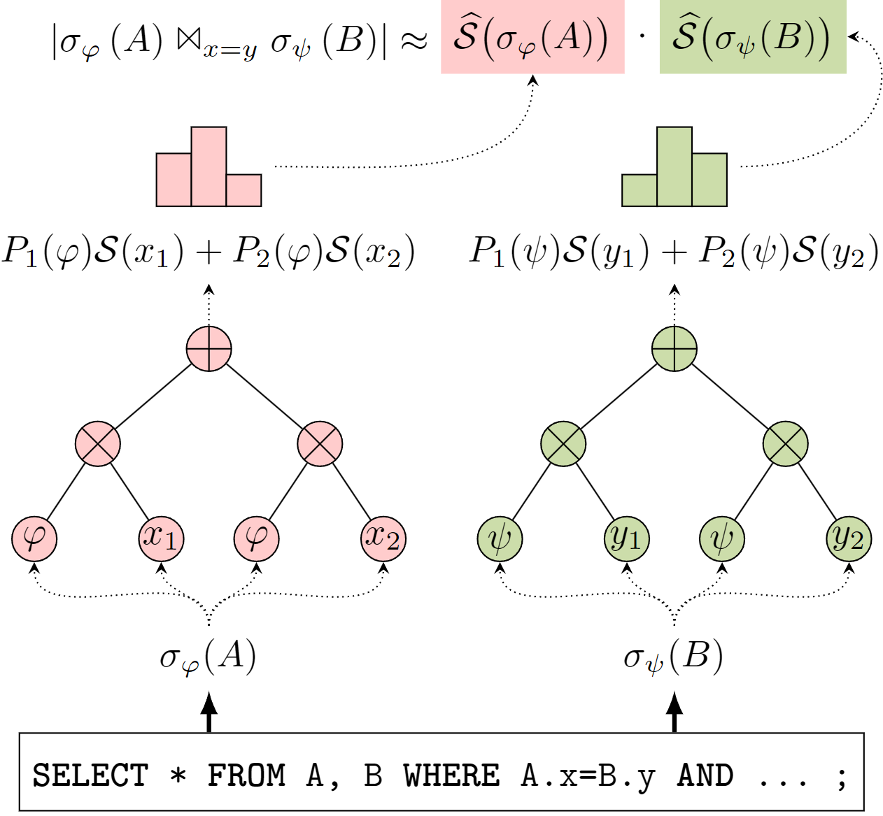
Error Bound for SPN Approximations
Conjecture: Approximation error is bounded by independence assumption
≤ ||sketch(σφ(T)) - sketch(T)×∏P(φᵣ)||₁
Worst-case: Single product node (full independence assumption)
Tighter independence/clustering thresholds → Closer to exact sketches
Upward-Biased Estimation
Observation: Overestimation is safer
- Underestimate → risky plans → catastrophic slowdown
- Overestimate → cautious plans → marginally suboptimal
Two Techniques for Upward Bias:
- Fast-AGMS Max: Take maximum instead of median
- Min-Product Node: Use min selectivity instead of product
- P(φ) × sketch → min{P(φᵢ)} × sketch
Experimental Results
Experimental Setup
Datasets:
- JOB-light: 70 queries (696 subqueries) on 6 IMDb tables
- Transitive joins, star schema, up to 5 tables
- Stats-CEB: 146 queries (2603 subqueries) on 8 Stack Exchange tables
- Non-transitive joins, more skewed/correlated data
Baselines:
- Exact Fast-AGMS and Bound Sketch
- DeepDB, BayesCard, FactorJoin, FLAT (learned estimators)
Sketch Approximation Error
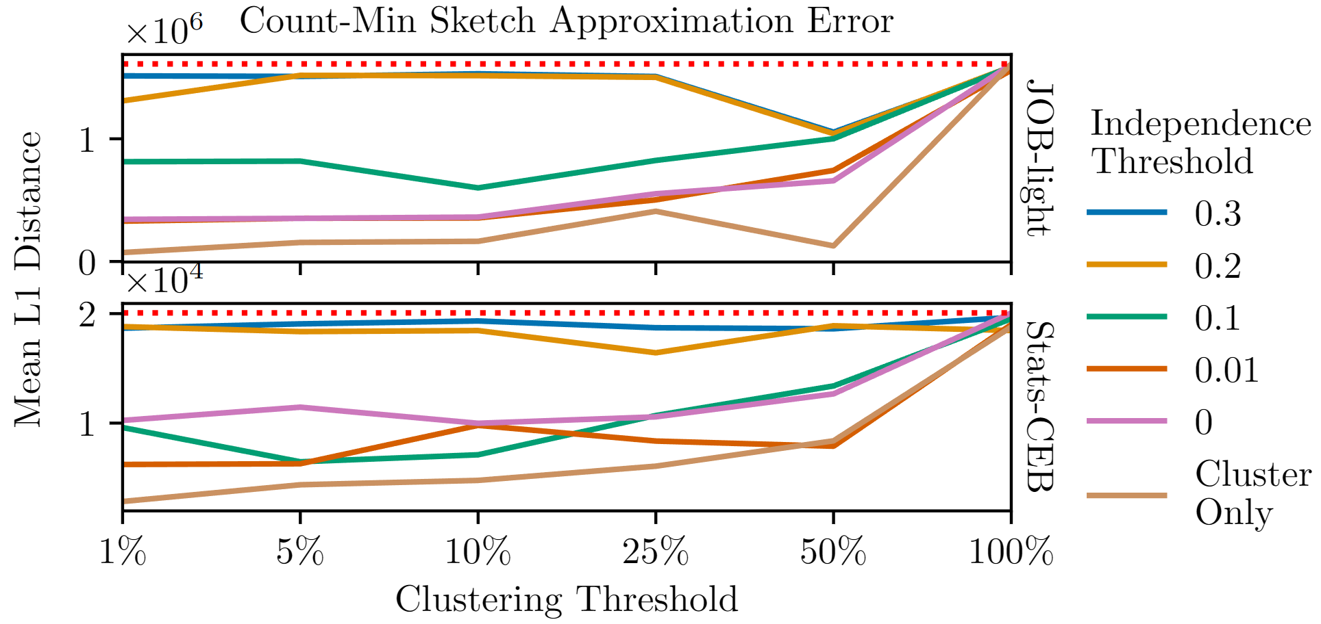
Takeaway: Just cluster, even a little bit, to drastically reduce error!
Approximation Efficiency
| Metric | Exact Sketches | Approximate Sketches |
|---|---|---|
| Sketch Construction Time | 737s (JOB-light) 155s (Stats-CEB) |
4.5s (JOB-light) 17.3s (Stats-CEB) |
| Space Required | 473 MB (JOB-light) 3.1 GB (Stats-CEB) |
1.2 GB model 676 MB model |
| Query Execution Time | 2.88 hrs (JOB-light) 9.16 hrs (Stats-CEB) |
2.88 hrs (0!) 9.31 hrs (+0.15) |
Within 3% of exact sketches! But much faster to compute.
Training Time Comparison
| Method | Model | JOB-light | Stats-CEB |
|---|---|---|---|
| Approximate Sketches | BERT | 148 min/epoch* | N/A |
| Sketched SPNs | SPN | 21 min | 2 min |
| DeepDB | SPN | 30 min | 55 min |
| BayesCard | Bayes Net | 6 min | 2 min |
| FactorJoin | Bayes Net | 4 min | 1 min |
*GPU required; others CPU-only
Sketched SPNs competitive with other per-relation methods
Model Complexity Trade-off
Query Execution Time
Exact F-AGMS would be the fastest, if not for construction time!
Model Comparison on JOB-light
BERT
- Limited by GPU memory
- Model size: 167 MB
- Training: 148 min/epoch
- Query Execution: 3.05 hrs
SPNs
- No GPU required
- Model size: 40 MB
- Training: 18 min total
- Query Execution: 2.93 hrs
Contributions Summary
Novel Contributions
1. Approximate Sketches (SIGMOD 2024)
- First application of neural networks to sketching
- Enables sketches for arbitrary filter conditions
- Bidirectional architecture handles any column ordering
2. Sketched Sum-Product Networks (2025)
- Scalability: larger sketches (no GPU bottleneck)
- Upward-bias: Fast-AGMS Max + Min-Product nodes
- Error bounds: worst-case = independence assumption
Impact on Query Optimization
Makes sketches practical
- No pre-computing sketches for selections
- No expensive query-time sketch construction
- Fast inference, suitable for optimization
- Scales to large databases (per-relation models)
Bringing It Together
1. Problem: Cardinality estimation is critical
2. Challenge: Joins are hard to estimate
3. Sketches: Fast, accurate, but limited
4. Our Solution: Learn distribution → Generate sketches
5. Results: Fast generation, high accuracy
Enables sketches for query optimization
without per-query construction!
Questions?
Brian Tsan
btsan@ucmerced.edu
Advisor: Professor Florin Rusu
UC Merced
Code & demos available at: github.com/btsan